Fast alle Rasenmähroboter verwenden eine Induktionsschleife (also einen geschlossenen Leiter von Punkt A nach Punkt B), um den Roboter auf das zu mähende Gebiet zu begrenzen – wie findet man aber die Stelle heraus, falls so eine Leitung einmal unterbrochen wurde? Ganz einfach: man baut sich einen “Cable Tracker” 🙂 …
Funktionsprinzip: Speist man eine Wechselspannung gegen Erde (als Masse) auf den unterbrochenen Leiter, so erzeugt diese ein elektrisches Feld um den Leiter. Dieses Feld kann man mit einer Spule detektieren. Wählt man für das Wechselsignal eine Frequenz von z.B. 400 bis 4000 Hz, so kann man dieses Signal um den Leiter herum mit einem kleinen Verstärker (z.B. Walkman) hörbar machen.
Verwendete Komponenten:
Der Sender:
Eine fertige PWM-Motor-Controller Schaltung (min. 30V), gefunden bei eBay (ist quasi ein fertiger Rechtecksignal-Frequenzgenerator mit Verstärker)
Ein Gleichstromnetzteil (30V – Achtung: auf keinen Fall mit höherer Spannung arbeiten)
Der Empfänger:
Eine Spule mit vielen Windungen aus einem alten 230V-Relais
Ein alter Walkman (oder Mikrofonverstärker)
Schritt 1: Den Senderaufbauen
Zunächst wurde der PWM-Controller mit nur 10Volt und einem Lautsprecher als “Motor” betrieben, und dabei die fertige PWM-Schaltung durch einen parallel ergänzten Kondensator so eingstellt, dass die Schaltung ein Rechteck-Signal mit gut hörbarer Frequenz erzeugt. Danach wurde der Lautsprecher entfernt, das Netzteil angeschlossen und als “Last” das offene Ende der Induktionsschleife und die “Rückführung” über einen Erdungsleiter (einfach ein Stahlrohr in die Erde gerammt).
Schritt 2: Der Empfänger
Ein alter Walkman wurde geöffnet und anstelle des Tonkopfes eine Spule angeschlosen. Wenn man nun den Walkman betreibt, hört man in der Nähe von Netzteilen/Steckdosen/etc. das typische 50 Hz Brummen – ein Zeichen dafür, dass der Empfänger funktioniert.
Schritt 3: Das Induktionskabel “abfahren”
Zum ersten Test nimmt man das Kabel für den Erdungsleiter einfach in die Hand (damit ist der abzufahrende Induktionskabel geerdet). Nun hört man in der Nähe (1-2 m) des Induktionskabels einen Ton, dessen Lautstärke durch Annäherung an das Kabel zunimmt. Genau an der Stelle der Unterbrechung hört der Ton auf und man hat die Stelle der Unterbrechung gefunden.
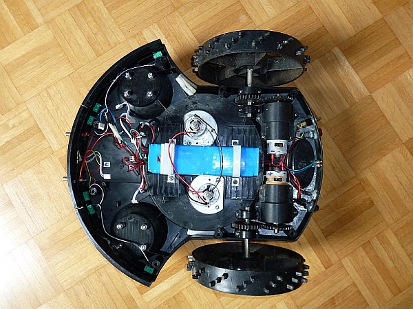
In the year 2009, I did purchase a Tianchen TC-G158 robot mower (via ChinaVasion) and this article describes some of the robot’s electronics internals, how to add an ultrasonic sensor to it, and how to connect your own microcontroller (e.g. Arduino) to the robot mower board so that you can write your own custom software for it. One primary warning already: Everything that includes opening your robot will loose your robot’s warranty. If you really need to do this (like me), be aware of this.
If you are talent enough, my material should give you a good start for your own experiments and adjustments – Happy mowing 🙂
–
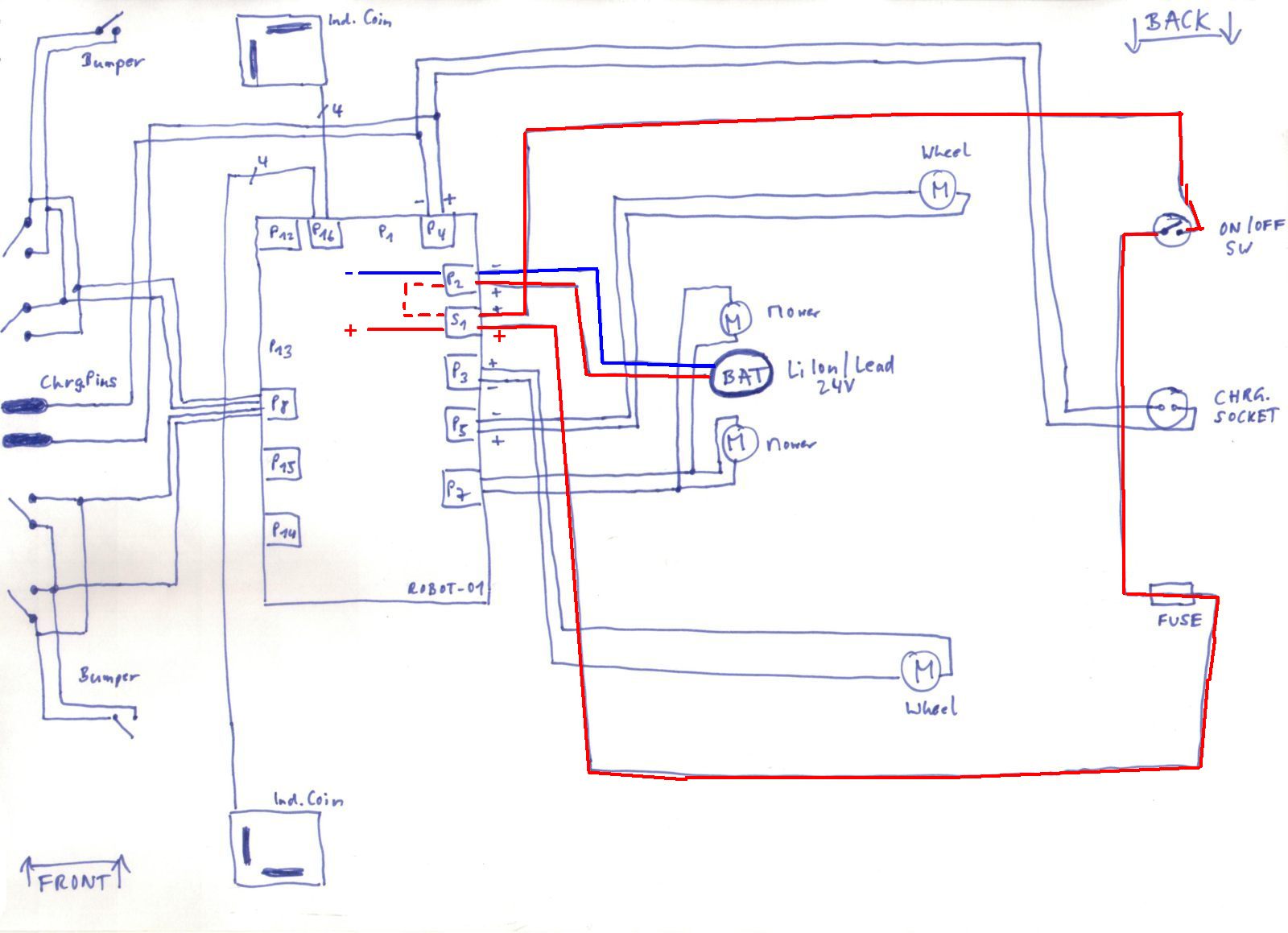
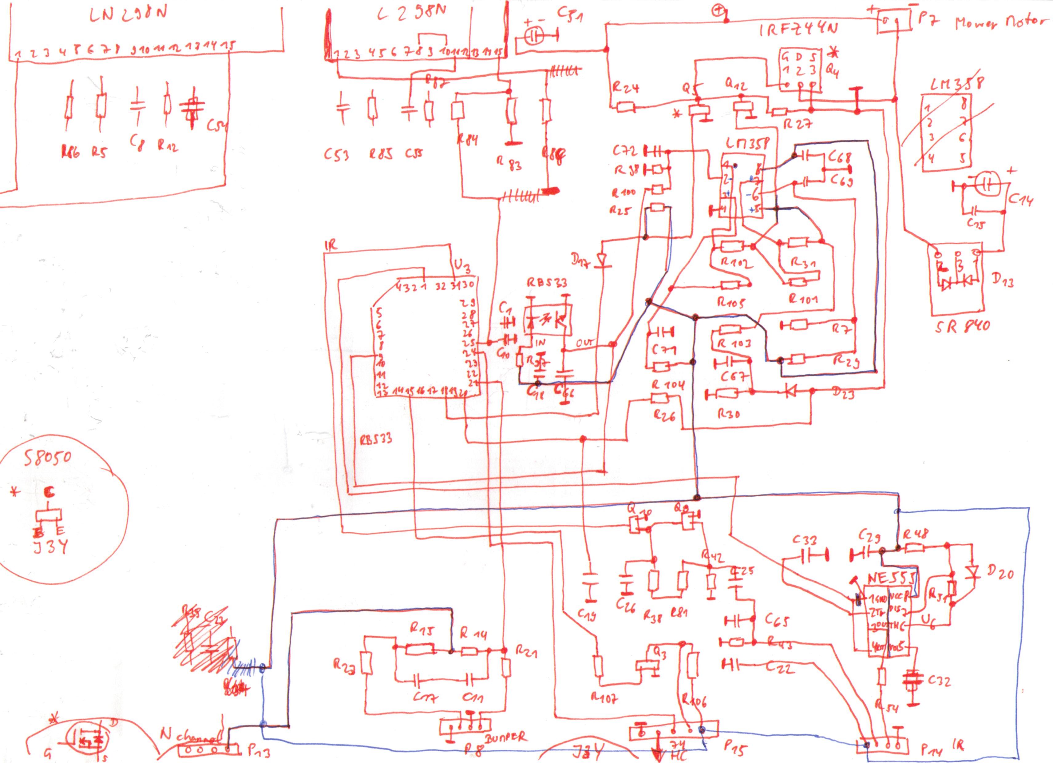
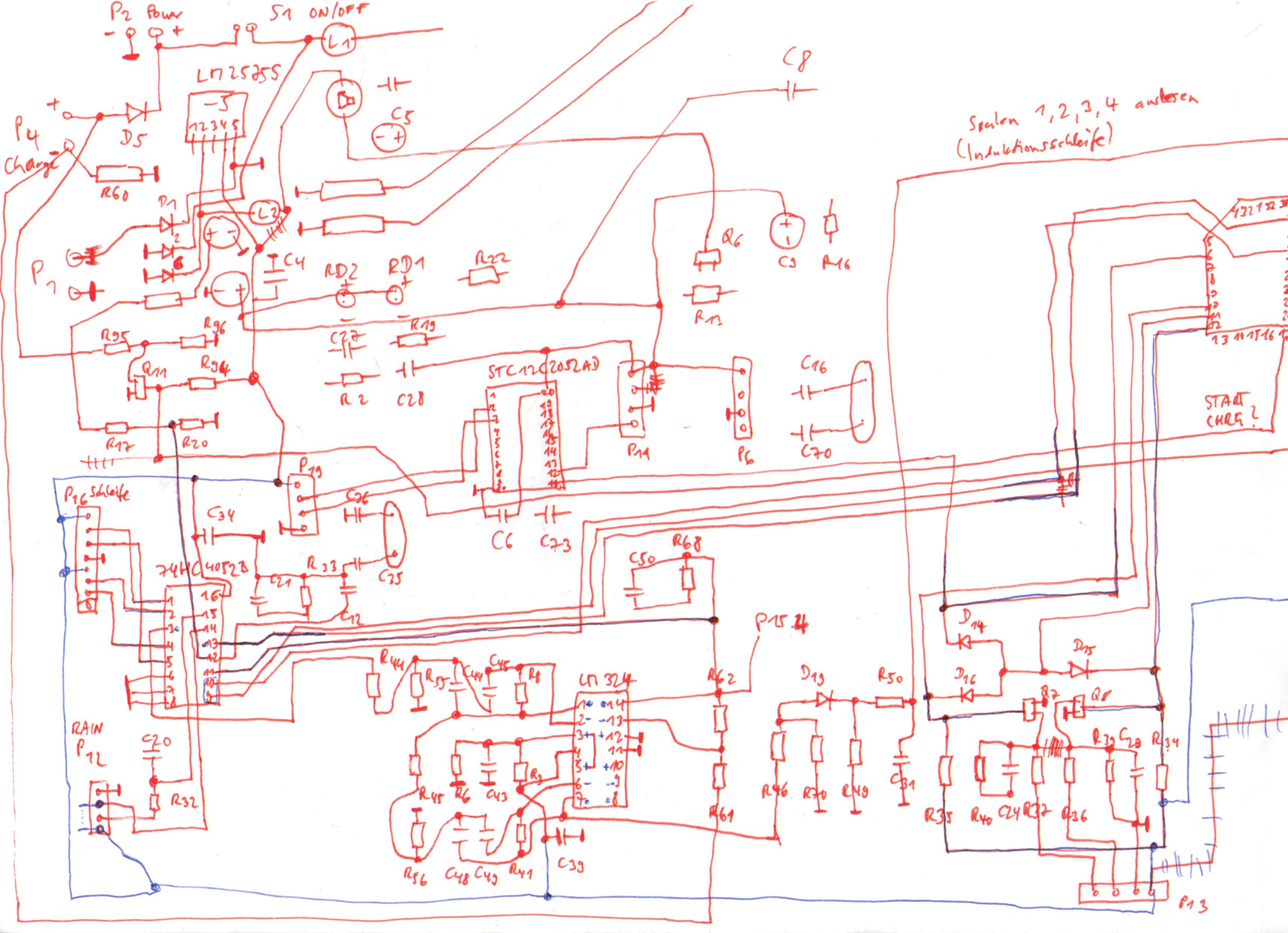
1. TC-G158 technical internals
This section should give you an overall idea of the components present in your mower. It’s good to roughly understand them for your own hacks!
My purchased Tianchen TC-G158 robot mower has the following components:
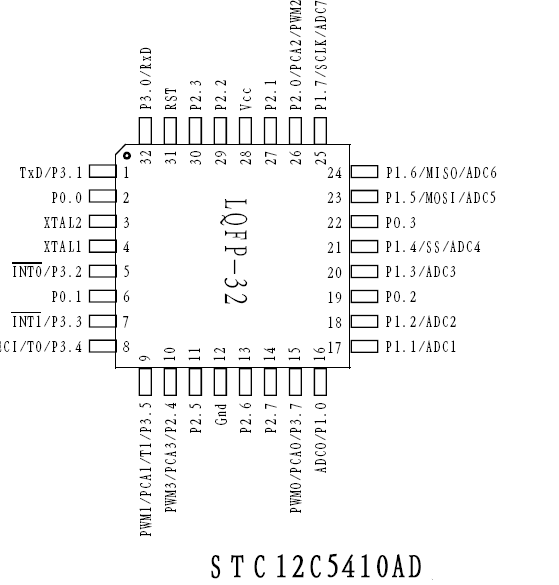
-Main MCU: STC12C5410AD (8051 clone, 10K flash memory, 33 Mhz)
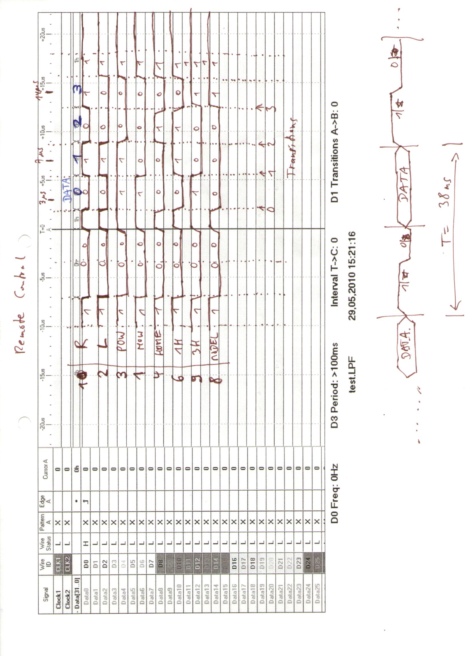
-Hope RF HM 433 Mhz receiver module (for remote control)
-Remote control decoder MCU: STC12C2052AD (sends remote control key data to main MCU, see protocol below)
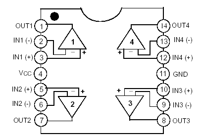
-Induction unit quad op amp: LM32 (for induction loop inductor amp)
-Optical roll ball sensor: HT RBS33 (theta=45 degree , switches off mowing motor above theta degree)
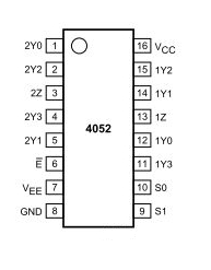
-Dual 4-channel mux/demux: 74HC4052D (to read in induction loop inductors and battery sense/rain sensor)
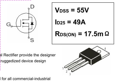
-Power MOSFET: IRFZ44N (for mowing motor)
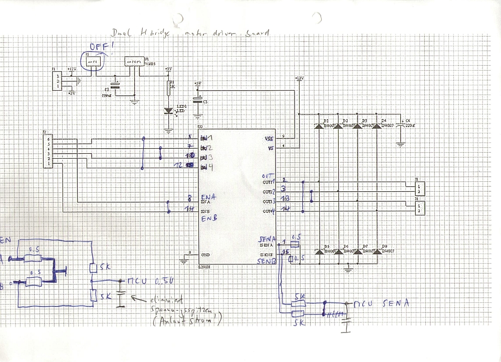
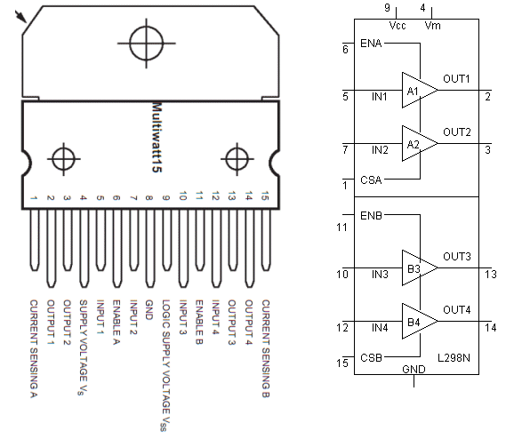
-Full bridge driver: L298N (for the left and right motors) – also see example schematics here
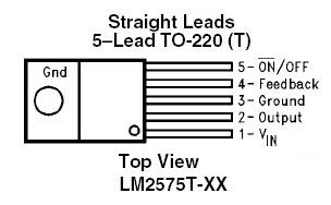
-1A step-down simple switch voltage regulator: LM2575S (for main board voltages)
-Solid state amp: SR840 (for mowing motor)
-Timer: NE555 (for IR modulation?)
-Dual op-amp: LM358 (for induction loop inductor)
–
2. Adding an ultrasonic sensor (Arduino hack)
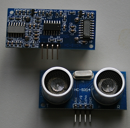
An ultrasonic distance sensor greatly helps to avoid bumping obstacles (or to drive into shrubberies). We use the HC-SR04 as it’s easy to use (you can find these boards on eBay).
This hack is universal – actually, you can add it to ANY robot mower. The good thing is you can keep the robot’s stock MCU firmware, and it’s easy to add: Just add another two wires to the front bumper push buttons, and your Arduino will simulate one of the bumpers (by switching the bumper signal to LOW) when the ultrasonic distance sensor detects an obstacle!
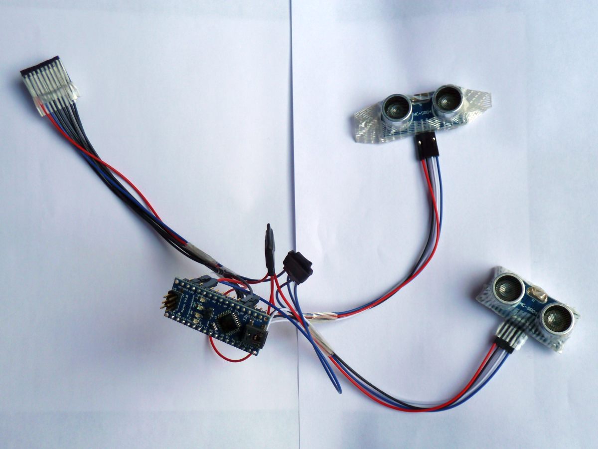
We use an Arduino Nano board for the controller as it’s very popular and very easy to program.
Arduino <—> robot wiring
Pin 7 <—-> robot left bumper signal pin (P8.2, see below)
Pin 8 <—-> robot right bumper signal pin (P8.4, see below)
Pin 12 <—-> ultrasonic board (trigger pin)
Pin 11 <—-> ultrasonic board (echo pin)
VCC <—-> robot +5V (P6.1, see below)
GND <—-> robot GND (P6.4, see below)
Robot bumpers pinout (P8) is (left-to-right):
1-GND
2-left bumper signal pin
3-GND
4-right bumper signal pin
Robot P6 pinout is (top-to-bottom):
1-VCC (+5V)
4-GND
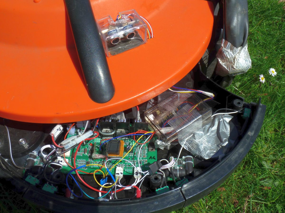
(the first photo shows the version for the Ambrogio L50 robot mower using two ultrasonic sensors)
For debugging purpose, you can add a piezo speaker:
Finally, you can see everything in action (NOTE: In this video, there is no perimeter that can stop the robot, it is only the ultrasonic sensor that can stop it)
NOTE: I have not tested yet how the ultrasonic sensor can be automatically deactived when the robot drives into the charging station – I’m not using any perimeter with this robot, so at least it works without perimeter…
For Arduino code, see resources section further below.
Hardware/software used for the hack:
A microcontroller that is easy to program: I did choose the Arduino Nano for all my hacks. You can find the Arduino Nano controllers on eBay (8-10 EUR)
Ultrasonic sensor board HC-SR04 – you can find those board on eBay (5-7 EUR)
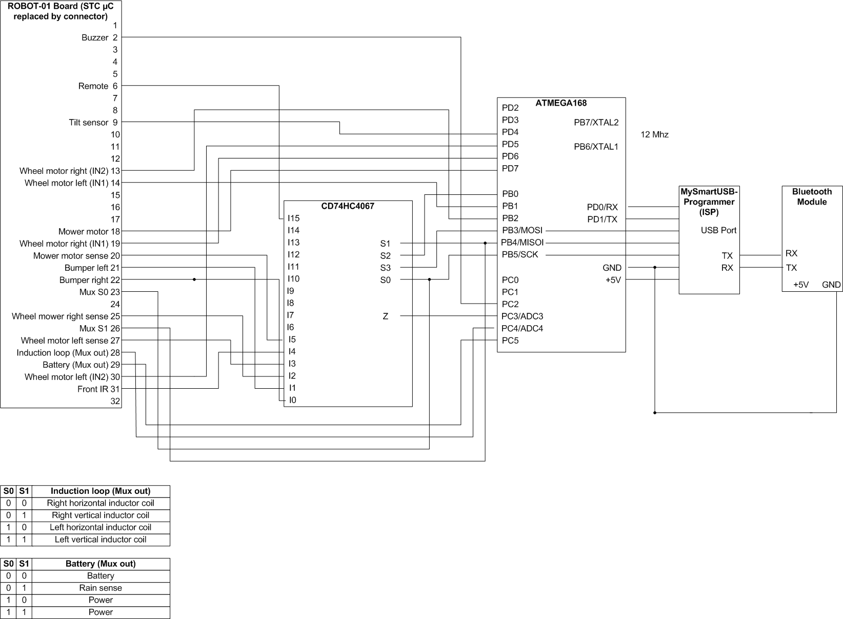
3. Replacing the stock MCU firmware (ATMEGA hack)
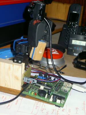
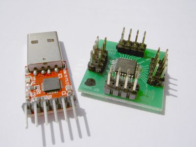
Replacing the stock MCU firmware requires to write a new firmware, and I did choose the Atmel ATMEGA-168 (on a ready myAVR board MK2 USB) as a replacement for the original 8051 MCU.
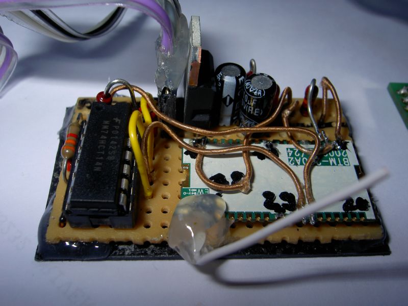
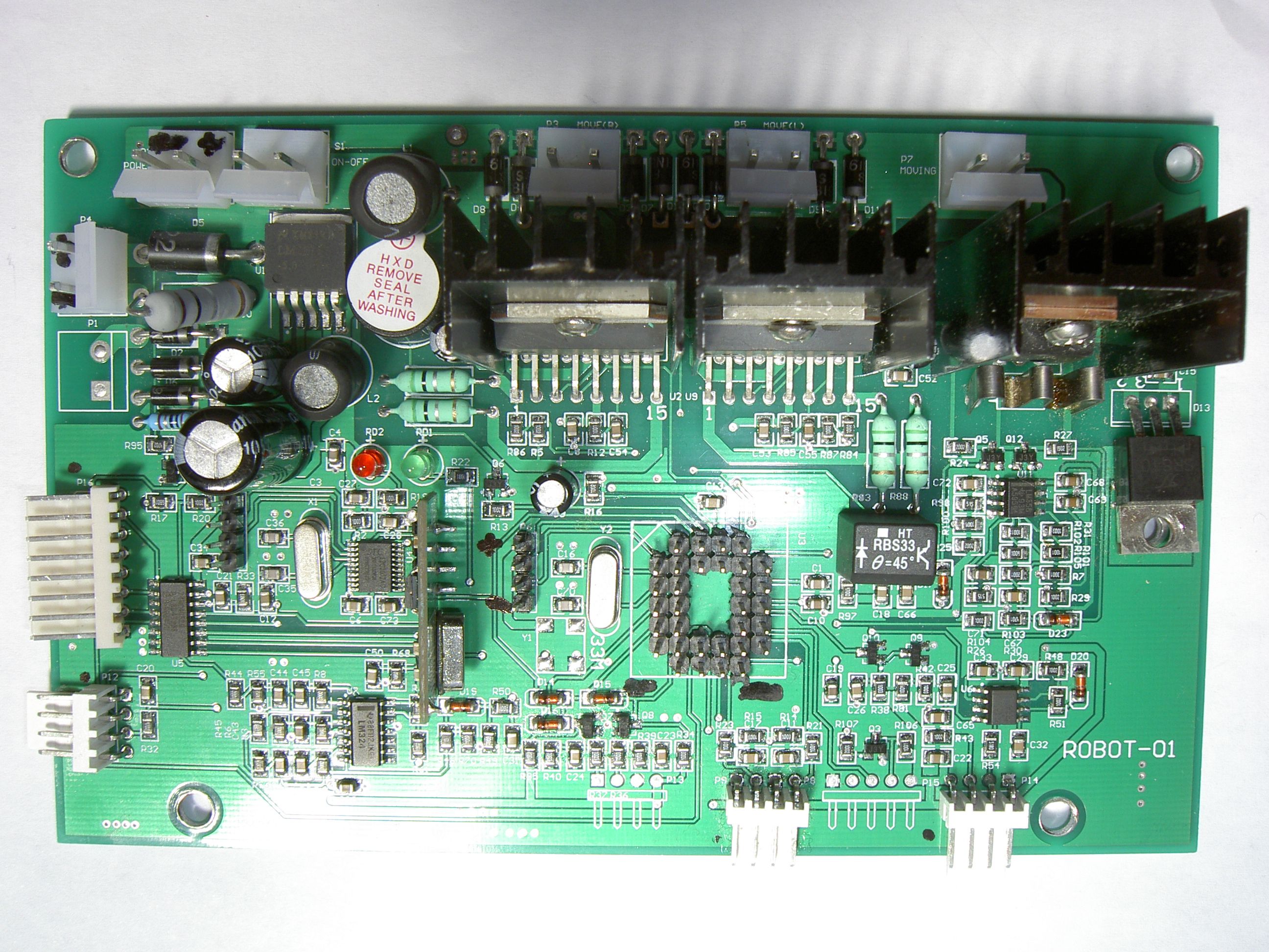
The first step is to desolder the MCU socket as you can see on my robot mower board .
Here you can see how I managed to connect my Atmel MCU to the old MCU socket (using some DIY adapter). Alternatively, you can directly connect the individual board pins to your Arduino board using 1-pin-cables (you can find them on eBay).
After a while, I noticed that I need something more fancy to upload my new custom software revisions into my mower while sitting comfortable in a chair meters away: a Bluetooth module! The bluetooth module extends the ordinary ISP RX/TX serial line (RS232) and also allows me to monitor sensor data and robot state changes (and believe me, this feedback is absolutely necessary for debugging your code…)
So this is my final system today:
Original board <==> ATMEGA168 <==> ISP (TTL UART) <==> Bluetooth module <~~> PC (Bluetooth dongle)
I upload new software builds into the mower via Bluetooth and the serial data of the mower is transmitted via Bluetooth too.
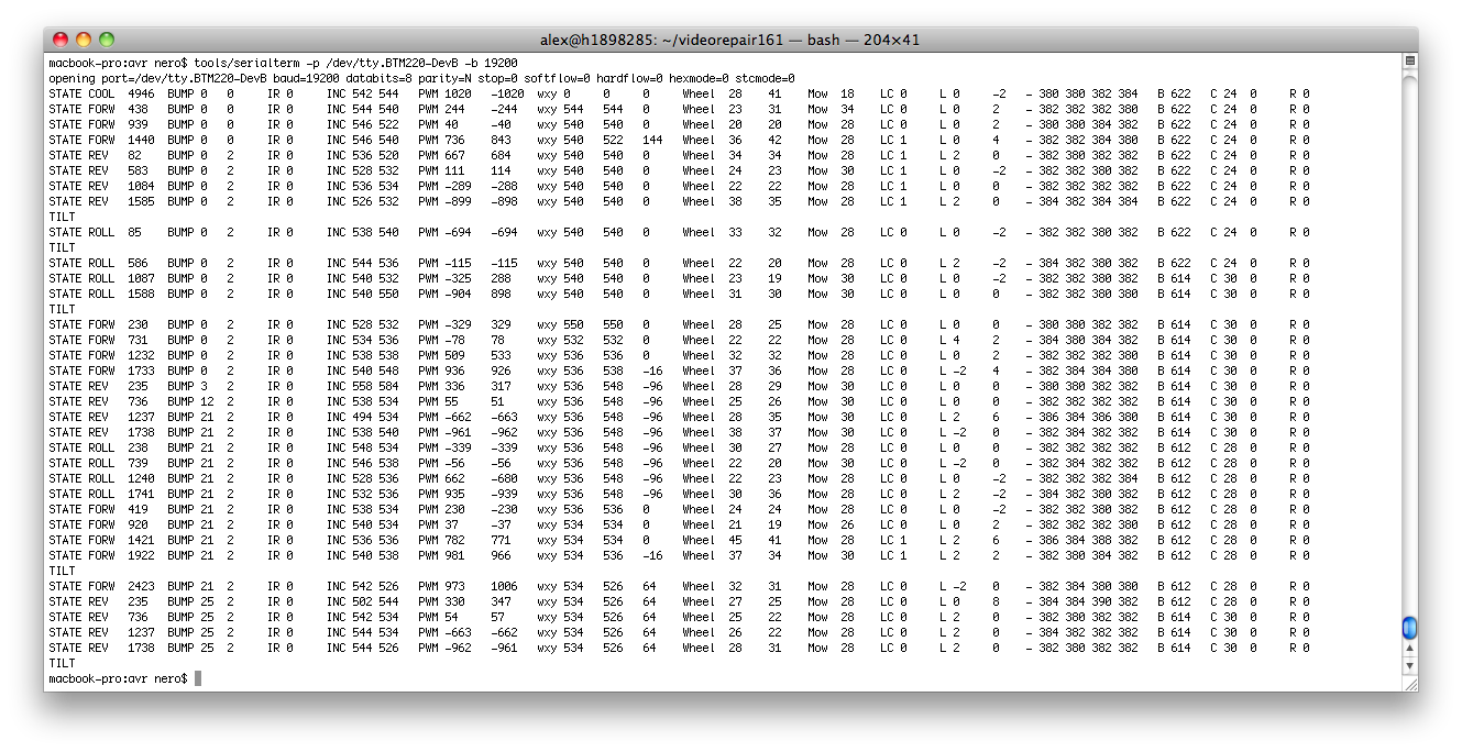
My latest software periodically displays the state of the mower (state, state time, bumper states, IR state, inclination sensor, motor PWM, motor PID controller wxy, motor current, induction coins values, battery state, rain sensor):
ATMEGA168 microcontroller (16K flash, operating at 5V)
12 Mhz oscillator
Bluetooth module BTM220 , an inverter 74HCT14N for level shift conversion (because my BTM220 operates at 3.3V, I needed a level shift conversion to 5V)
Multiplexer CD74HC4067 (to reduce the number of required pins at the microcontroller)
Two photo sensors to measure the wheel movement (wheel left/right balance control) – later I replaced this by a declination sensor which works great too
For ATMEGA code, see resources section further below.
–
4. Adding a PID controlfor the wheels
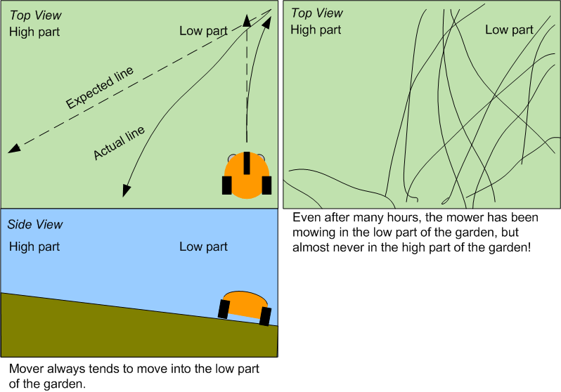
After purchasing, I noticed the robot has a small problem: when moving from the lower part to the higher part of my garden, it doesn’t move a straight line – it makes circles of 90 degress and less (due to the heavy lead acid batteries my mower is using) …
(Also have a look at my mower simulation that demonstrates the difference ‘lawn with and wihtout slope’).
So I decided to add some software PID controller to it to control the left-right wheel balance 🙂 and it solved this specific problem (see videos with and without balance controller).
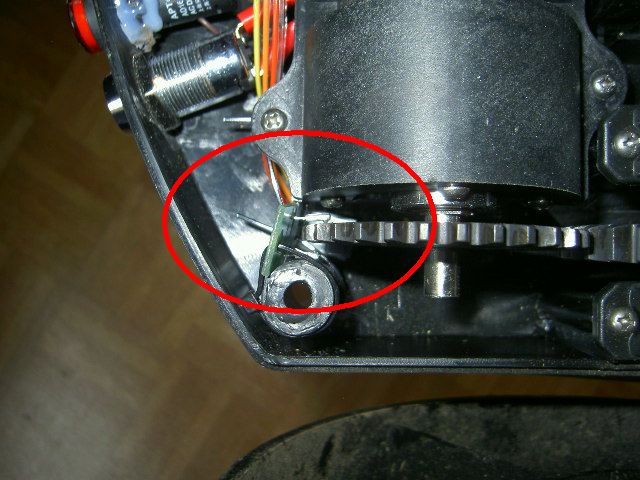
And here you can see how I added photo interruptors (LTH301-07) for the left and right motors to measure the wheel movement (for the left-right wheel balance control):
My pseudo-schematics (1), (2)
(Warning: always measure and verify using your own board – manufacturers often change their layouts and make adjustments, and without measuring you may damage your own board!)
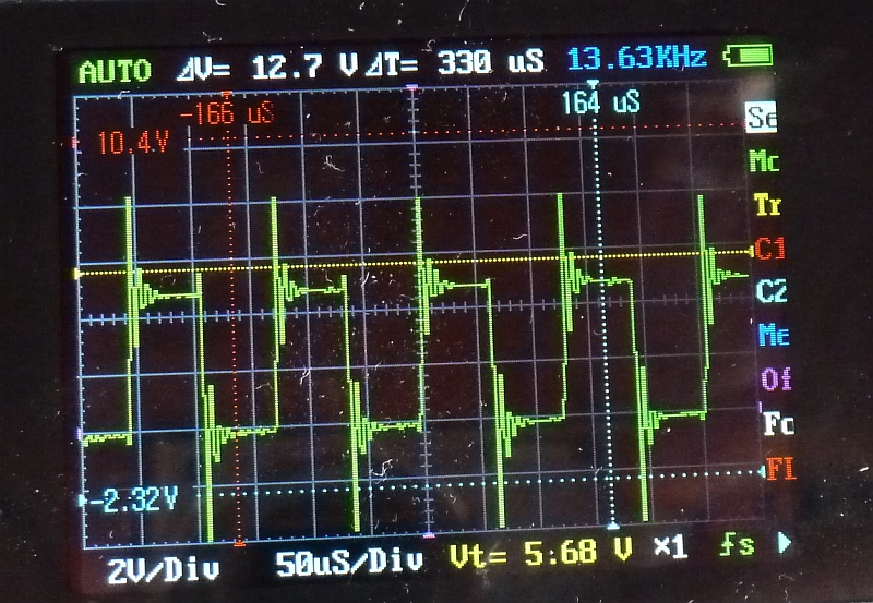
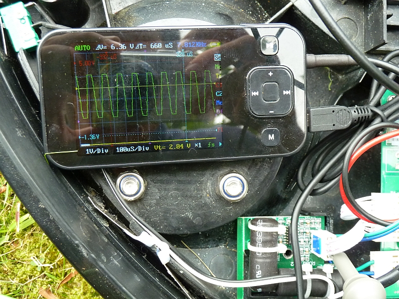
Charger induction loop signal (measured at induction loop cable output)
Induction loop coil signal (measured at induction coil connector)
Connector pinout: +5V, GND, vertical coil output, horizontal coil output
ATMEGA robot mower code (code also describes the MCU socket<->ATMEGA168 wiring – Warning: don’t expect this code to work at once in your own configuration – you’ll need to study schematics, your MCU specifications and much more to get it working!)
Pinout of ICs LM2575S(voltage regulator) IRFZ44N(N channel power MOSFET) LM324(operation amplifier) 74HC4052(multiplexer) L298N (motor driver) STC12C5410AD(MCU)
STC5406AD (MCU)
–
6. External resources on the Internet
Wiring diagram for the updated version of the robot (additional security board) which turns-off the mower when the front wheels have no contact
Induction loop receiver board schematics (and more) at robi2mow
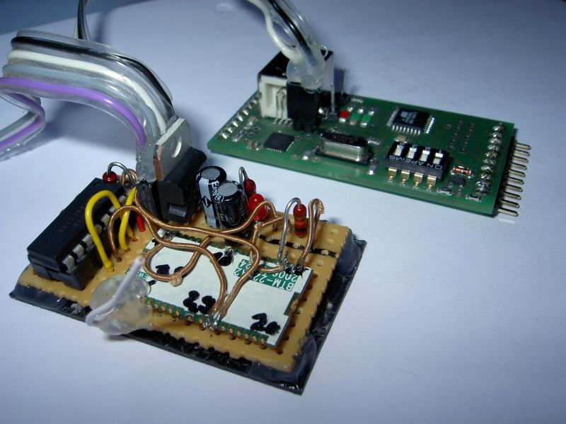
Dieser Artikel beschreibt, wie man ein Bluetooth-Modul mit einem ISP-Programmer (hier: das ‘mySmartUSB-Modul’ der Firma Laser & Co. Solutions GmbH) verbindet und auf diese Weise Mikrocontroller via Bluetooth mit dem PC programmieren und zusätzlich Daten mit dem Mikrocontroller und dem PC austauschen kann. Diese Möglichkeit, beides kabellos zu bewerkstelligen (Mikrocontrollerprogrammierung -und RS232-Datentransfer) , dürfte relativ einzigartig sein!
Ausgangslage
Manchmal wäre es ‘Nice-to-have’, manchmal geht es aber auch nicht anders: man möchte das Kabel zwischen Mikrocontroller und PC loswerden. In unserem Fall sollte ein mobiler Roboter per Funk vom PC programmiert und später dessen Sensordaten im Betrieb an diesen PC übertragen werden.
Warum überhaupt Bluetooth?
es gibt kostengünstige USB-Bluetooth-Dongles für den PC (wenige Euro) (PC-seitig braucht man also nichts entwickeln!)
Bluetooth simuliert eine serielle Schnittstelle (COM-Port) am PC – man kann also alle bisherigen Tools und Programme weiterverwenden (PC-seitig bleibt also alles beim Alten!)
die Reichweite ist akzeptabel (100-150 m , Bluetooth class1)
es gibt kostengünstige (ca. 15 €) Bluetooth-Module mit 3.3V TTL UART-Schnittstelle (4 Pins werden davon benutzt: 3.3V VCC, GND, TX und RX)
Warum mySmartUSB als ISP-Mikrocontroller-Programmer?
er unterstützt die gängigsten Programmierprotokolle (AVR910/AVR911)
einziger ISP-Programmer (meines Wissen), der auch als UART-Bridge fungieren kann und diese ist dazu auch noch per UART-Kommando schaltbar(!) (mehr dazu unten) – den USB-zu-UART Konverter (CP2102) brauchen wir hier jedoch nicht
Verwendete Komponenten
myAVR mySmartUSB (v2.10) zur µC-Programmierung/UART Datentransfer mit diesem
myAVR Board mit ATmega168
Bluetooth-Modul BTM220
3.3V Spannunsgregler (LF33CV), 2 Elkos, 4 Widerstände, 1 LED, 1 IC (74HCT14N) für den Bluetooth-Adapter
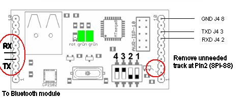
Schritt 1 : Bluetooth-Adapter für mySmartUSB bauen
Für diesen Zweck wird hier das Rayson Bluetooth-Modul ‘BTM220A’ verwendet, welches eine UART-Schnittstelle verwendet. Da dieses Modul jedoch mit 3.3V Spannungsversorgung arbeitet, wird ein 3.3V Spannungsregler sowie ein 3.3V zu 5V TTL Pegel-Wandler (für RX/TX) eingesetzt. Die genaue Adapter-Schaltung kann z.B. dem Blog von Martin Hänsler entnommen werden. Zur Pegel-Wandlung der TX- bzw. RX-Leitungen wird dort ein invertierendes Schmitt-Trigger IC verwendet, ein Spannungsteiler sorgt bei der RX-Leitung für den 3.3V Level.
Nach einer nachmittaglichen Bastelarbeit könnte das vollständige Bluetooth-Modul dann z.B. so aussehen 🙂
Ergebnis: Bluetooth-Modul mit 5V TTL UART (mit vier Anschlußpins: 5V VCC, GND, TX und RX)
Schritt 2 : TX und RX am mySmartUSB suchen
Im nächsten Schritt soll mit diesem Bluetooth-Modul ein ATmega168 auf einem myAVR Board programmiert werden können (natürlich über Bluetooth). Zusätzlich soll aber auch das ATmega UART-Modul mit dem PC über Bluetooth angebunden werden, so dass man kabellos Daten mit dem Mikrocontroller austauschen kann. Für beide Zwecke bietet sich die ‘mySmartUSB-Tocherplatine‘ des myAVR-Boards geradezu an, da es über einfache UART-Kommandos zwischen Programmier- und Datenmodus umschalten kann.
Ein Problem muss allerdings noch gelöst werden: der Programmer verfügt offensichtlich nur über einen USB-Anschluß als Programmierschnittstelle, die TX/RX-Leitungen zum Programmer hin müssen also ausfindig gemacht werden -vom CP2102-USB-zu-seriell Konverter Baustein ausgehend findet man RX an Pin5 und TX an Pin4 der mySmartUSB-Steckpfosten links:
(Anmerk.: in der mySmartUSB Dokumentation findet man nur die rechten TX und RX Pins für die UART-Bridge – diese können aber nicht zum programmieren sondern nur für den Datenaustausch verwendet werden).
Die benötigte 5V Spannungsversorgung für den Spannungsregler des Bluetooth-Moduls muss man sich ggf. über das myAVR-Board holen – ohne USB-Anschluß scheint der Programmer nur etwa 4V über das myAVR-Board zu bekommen.
Schritt 3 : mySmartUSB und Bluetooth-Adapter verbinden
Dann kommt der spannende Augenblick beide Module miteinander zu verbinden 🙂
Wichtig: RX vom Bluetooth-Modul geht auf TX vom mySmartUSB (was der eine sendet, muss der andere empfangen)
Und siehe da! Ein erstes Austesten mit den bisherigen myAVR-Tools und Programmen zeigt : alle Funktionen laufen wie erwartet!
Im nächsten Schritt werde ich wohl die mögliche Reichweite dieses Bluetooth-Moduls austesten – 100 Meter im Freien sollten damit machbar sein 🙂
Fazit: …ich bin mir sicher: so ein fertig aufgebautes Bluetooth-Modul wäre garantiert eine ideale Ergänzung des myAVR-Sortiments 😉
Endlich mal wieder ein kleines Projekt, welches viele Dinge der Informatik miteinander verbindet: Servos, Mikrocontroller, USB-Kamera, Mikrocontroller <-> PC-Kommunikation, HTTP-Server, Javascript, AJAX, Python …
Aber jetzt erstmal im Detail:
Wie der Titel schon andeutet, geht es darum, eine USB-Webcam, welche auf zwei Servos montiert wurde via einem Web-Interface fernzusteuern – und natürlich das Bild der Kamera zu übertragen.
Das Projekt ist ähnlich dem Projekt von Tobias Weis – allerdings wird hier Windows und als Skriptsprache Python (statt Linux und PHP) verwendet.
Funktionsweise
Die Servos werden über Pulsweitenmodulation (PWM) vom Mikrocontroller angesteuert, der Mikrocontroller erhält die Steuerbefehle via RS232-Schnittstelle (RS232 through USB). Ein auf dem PC laufender und in Python geschriebener Web-Server liest regelmäßig Bilder von der USB-Kamera, nimmt Befehle vom Web-Client entgegen (Kamera nach rech/links/oben/unten) und schickt diese Befehle dann an den Mikrocontroller.
Benötigte Hardware
Mikrocontroller Atmel ATMEGA8L (ich verwende das myAVR Board MK2 USB von myAVR) – dieses Board enthält den Mikrocontroller sowie einen Programmer zum Übertragen der Software in den Mikrocontroller via USB.
2 handelsübliche Servos (werden im Modellbau eingesetzt und gibt es teilweise recht günstig bei eBay – ansonsten beim Modellbauer, Conrad, …)
USB-Webcam (gibt’s überall)
Ein Netzteil (5V, ca. 1A) zur Energieversorgung der Servos
Benötigte Software
Atmel AVR Studio 4 (kann man bei Atmel herunterladen) – zum Kompilieren/Übertragen der Mikrocontrollersoftware
Python 2.6 – Skriptspraceh zum Ausführen des Web-Servers, Kamera-Zugriff, Mikrocontroller-Kommunikation etc.
Schritt 1: Servos montieren und mit Mikrocontroller verbinden
Den ersten Servo auf ein Brett fixieren, den zweiten Servo auf den ersten montieren und die Kamera auf den zweiten Servo befestigen. Dann die Steuerleitungen der Servos mit den Atmel Pins PB1 (OC1A) und PB2 (OC1B) verbinden. Zuletzt die +5V und Masse-Leitung der Servos mit dem externen Netzteil verbinden und die Masse-Leitung des externen Netzteils mit der Masse des Atmels verbinden (siehe auch das Schaltbild von Tobias).
Schritt 2: Mikrocontroller programmieren
Als nächstes wird der Atmel-Mikrocontroller programmiert. Zunächst sicherstellen dass die Fuse Bits des Atmels so eingestellt sind, dass dieser mit dem externen 3.6864 Mhz Quartz arbeitet (wichtig für die RS232 Kommunikation), z.B. mit dem Tool AVROSPII. Dann die Mikrocontroller-Software (avr/test2.c bzw. Projektdatei avr/test2.aps) in den Atmel mit AVR Studio übertragen (Build->Build und danach Tool-AVR Prog). Falls das myAVR-Board nicht gefunden wird, überprüfen ob COM1 oder COM2 für den USB-Treiber (->Gerätemanager) verwendet wird.
Nach erfolgereicher Übertragung der Mikrocontroller-Software kann man die Servos mit der Batch-Datei (avr/term.bat) austesten, welche ein RS232-Terminal startet. Durch Drücken der Tasten 1, 2, 3 oder 4 kann man die Servos steuern (rechts/links/oben/unten).
Schritt 3: Web-Server starten
Die WebCam mit dem PC verbinden. Dann den Web-Server starten (im Verzeichnis control ausführen: python start.py). Nach ein paar Sekunden läuft der Web-Server dann auf Port 8080. Im Web-Browser gibt man also “http://localhost:8080” als URL ein und mit ein bisschen Glück sieht man das Web-Interface der Steuerungssoftware.
This video shows our prototyped flight simulation and controller software that
simulates the flight dynamics of an RC aircraft and
automatically controls that aircraft so that it avoids obstacles (ground/mountains etc.), only by analysing the optical flow in front of the aircraft. For the optical flow sensor, an optical mouse CCD (20×20 pixels) with a lense is simulated.
Also click here to see how the same technique is used in 2D to navigate a robot, only by optical flow.
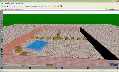
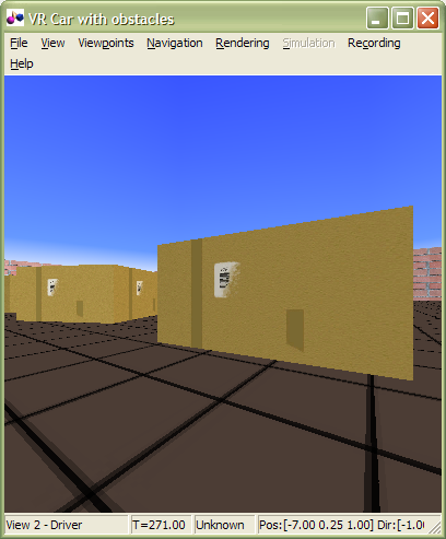
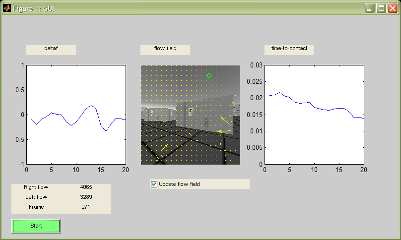
This is the result of a project where a virtual robot avoids obstacles in a virtual environment without knowing the environment – the robot navigates autonomously, only by analysing it’s virtual camera view.
In detail, this example project shows:
1. How to create a virtual environment for a virtual robot and display the robot’s camera view
2. Capture the robot’s camera view for analysing
3. Compute the optical flow field of the camera view
4. Estimate Focus of expansion (FOE) and Time-to-contact (TTC)
5. Detect obstacles and make a balance decision (turn robot right/turn left)
Matlab’s Virtual Reality toolbox makes it possible to not only visualize a virtual world, but also capture it into an image from a specified position, orientation and rotation. The virtual world was created in VRML with a plain text editor and it can be viewed in your internet browser if you have installed a VRML viewer (you can install one here).
(Click here to view the VRML file with your VRML viewer) .
For calculating the optical view field of two successive camera images, I used a C optimized version of Horn and Schunk’s optical flow algorithm – see here for details).
Based on this optical flow field, the flow magnitudes of right and left half of each image is calculated. If the sum of the flow magnitudes of the view reaches a certain threshold, it is assumed there is an obstacle in front of the robot. Then the computed flow magnitude of right and left half image is used to formulate a balance strategy: if the right flow is larger than the left flow, the robot turns left – otherwise it turns right.
Did you know that a fly cannot see real stereo? It sees two “images” that have only a small area of the same visual field. So the fly cannot estimate distances by using stereo images, it detects obstacles by “optical flow”. Optical flow is the perceived visual motion of objects as the observer (here the fly) moves relative to them.
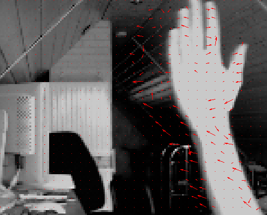
I have experimented with optical flow code (based on Horn and Schunck’s optical flow algorithm) these days, and I could manage to visualize the optical flow with it in real-time using 100% Matlab code. The code uses a camera (320×240 pixels) for capturing real-time image frames, computes the optical flow field with the current and the last frame (also called image velocity field) and shows the field in the image.
The field is calculated for each pixel of the image. The angle of the arrow shows in which direction the specified pixel was moved, the distance shows how much that pixel did move.
How can this optical flow field be used? Well, you could e.g. use the field to estimate the distance to obstacles for a moving vehicle when mounted a camera on it. A nice approach of detecting obstacles for a robot vehicle 🙂
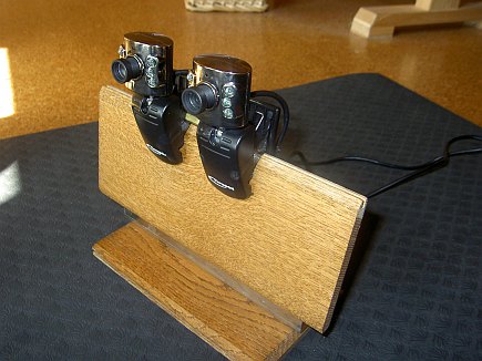
The aim of this project is to experiment with a self-made USB stereo vision camera system to generate a depth-map image of an outdoor urban area (actually a garden with obstacles) to find out if such a system is suitable for obstacle detection for a robotic mower. The USB camera I did take (Typhoon Easycam 1.3 MPix) is very low priced (~12 EUR) and this might be the cheapest stereo system you can get.
For the software, the following steps are involved for the stereo vision system:
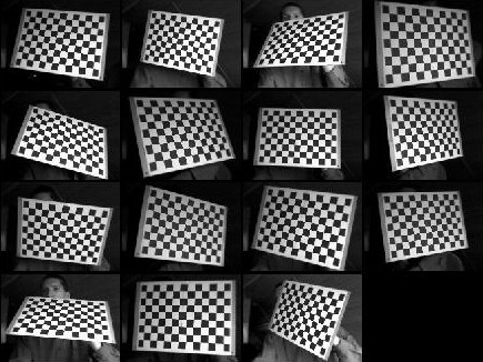
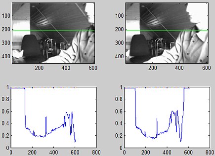
1. Calibrate the stereo USB cameras with the MATLAB Camera Calibration Toolbox to determine the internal and external camera paramters. The following picture shows the snapshot images (left camera) used for stereo camera calibration.
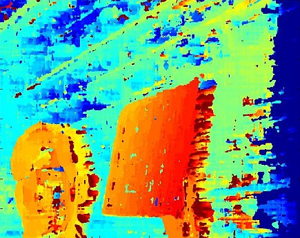
2. Use these camera paramters to generate rectified images for left and right camera images, so that the horizontal pixel lines of both cameras contain the same obstacle pixels. Again, the mentioned calibration toolbox was helpful to complete this task since rectification is included.3. Find some algorithm to find correlations of pixels on left and right images for each horizontal pixel line.This is the key element of a stereo vision system. There are algorithms that produce accurate results and they tend to be slow and often are not suitable for realtime applications. For my first tests, I did experiment with the MATLAB code for dense and stereo matching and dense optical flow of Abhijit S. Ogale and Justin Domke whose great work is available as open-source C++ library (OpenVis3D). Running time for my test image was about 4 seconds (1.3 GHz Pentium PC).4. Compute the disparity map based on correclated pixels.My test image:
The disparity map generated (from high disparity on red pixels to low disparity on blue pixels):
The results are already impressive – future plans involve finding faster algorithms, maybe some idea that solves the problem in another way. Finding a quick way to find matches (from left to right) in intervals between the left and right intensity scan lines for each horinzontal pixel line could be a solution, although it might always be too slow for realtime applications.
Update (06-17-2009): I have been asked several times now how exactly all steps are performed. So, here are the detailed steps:
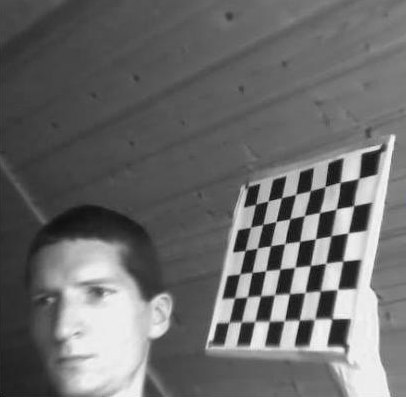
Learn how to use the calibration toolbox using one camera first. I don’t know how to calibrate the stereo-camera system without the chessbord image (anyone knows?), however it is very easy to create this chessboard image – download the .PDF file, print it out (measure the box distances, vertical and horizontal line distances in each box should be the same), and stick it onto a solid board. Calibrate your stereo-camera system to compute your camera parameters. A correct calibration is absolutely necessary for the later correlation computation. Also, check that the computed pixel reprojection error after calibration is not too high (I think mine was < 1.0). After calibration, you’ll have a file “Calib_Results_stereo.mat” under the snapshots folder. This file contains the computed camera paramters.
Now comes the tricky part 😉 – In your working stereo camera system, for each two camera frames you capture (left and right), you need to rectify them using the Camera Calibration Toolbox. You could do this using the function ‘rectify_stereo_pair.m’ – unfortuneately, the toolbox has no function to compute the rectified images in memory, so I did modify it – my function as well as my project (stereocam.m) is attached.Call this at your program start somewhere:
rectify_init
This will read in the camera parameters for your calibrated system (snapshots/Calib_Results_stereo.mat) and finally calculate matrices used for the rectification.
Capture your two camera images (left and right).
Convert them to grayscale if they are color: imL=rgb2gray(imL)
imR=rbg2gray(imR)
Convert the image pixel values into double format if your pixel values are integers:
imL=double(imL)
imR=double(imR)
Rectify the images:
[imL, imR] = rectify(imL, imR)
For better disparity maps, crop the rectified images, so that any white area (due to rotation) is cropped from the images (find out the cropping sizes by trial-and-error): imL=imcrop(imL, [15,15, 610,450]
imR=imcrop(imR, [15,15, 610,450]
The rectified and cropped images can now be used to calculate the disparity map. In my latest code, I did use the ‘Single Matching Phase (SMP)’ algorithm from Stefano, Marchionni, Mattoccia (Image and Computer Vision, Vol. 22, No .12): [dmap]=VsaStereoMatlab(imL’, imR’, 0, Dr, radius, sigma, subpixel, match)
Do any computations with returned depth map, visualize it etc.
And finally, here’s the Matlab code of my project (without the SMP code).
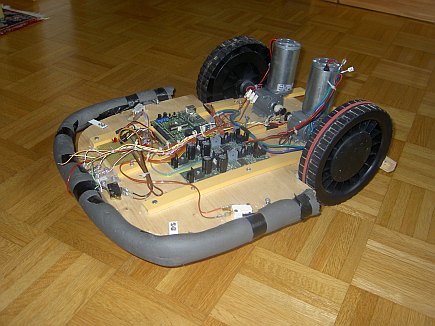
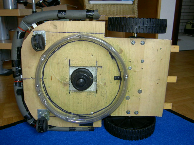
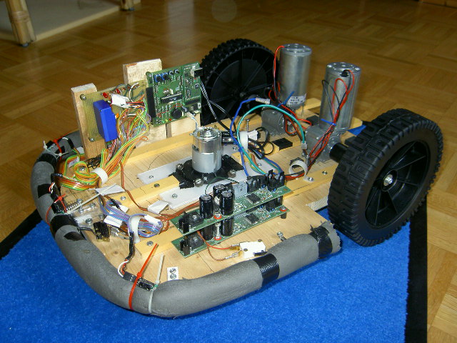
Wouldn’t it be nice to lie in the sun and have a robotic mower mow the lawn (and do the boring work)? Well, at least this is the aim (among other aspects as learning more about designing such systems) of this project…
A) Mechanics
Two wheels of a seed vehicle
Two office chair front wheels
Two DC motors motors (12V, 40W) with gear (23:1)
B) Mowing unit
DC motor from a 18V battery lawn trimmer
C) Controller
Microcontroller board ATMEGA168 (myAVR, 50 EUR) for reading the sensors and controlling the motors (two rear motors).
D) Sensors
Three Sharp IR sensors to detect near obstacles
RGB color sensor to detect non-lawn/lawn areas (no need to build a virtual fence in your garden!)
Bumper with three micro switches
E) All other parts
A wooden board (38 x 53 cm) for assembly of everything
Two gel-lead batteries (2 x 12V, 10Ah)
F) First version (without mowing unit), without sensors
Click here to see video (9 MB) which shows this mower prototype in action (indoor) 🙂 G) Second version – now with sensors and mowing unit!
The color sensor is working – the RGB color value is measured periodically and then converted into HSV (hue/saturation/value) color model. A first test with real lawn shows it can detect areas with a green color very precisely. For testing the algorithm, the first goal was to keep the robot on the blue piece of carpet – it successfully stayed on there, even after ‘mowing’ for 30 minutes!
A blog on projects with robotics, computer vision, 3D printing, microcontrollers, car diagnostics, localization & mapping, digital filters, LiDAR and more


