( applications requiring advanced vehicle dynamic control in real-time )

This blog article introduces the basics to use ACADO toolkit from Python as an MPC controller for a robotic car. For this example we will write a ACADO-Python extension for the AtsushiSakai Python Robotics example ‘model_predictive_speed_and_steer_control.py‘. The ACADO toolkit will generate very fast MPC controllers (that perform one control step in microseconds) that can be used for realtime MPC control. The goal for the MPC controller is to autonomously steer a robot car on a reference course (reference trajectory).

Control Theory

State varibles: The smallest possible subset of system variables that can represent the entire state of the system (robot, plant, rocket etc.) at any given time.

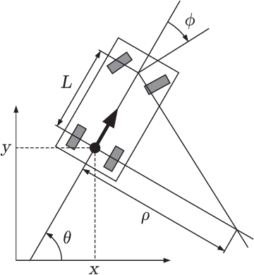
Example for a car (aka bicycle model – see below car drawing):
state vector: [x, y, v, phi]

(x: the x position [m], y: the y position [m], v: vehicle speed in [m/s], phi: vehicle orientation [rad])
NOTE: For our car example, the black dot is the control point, so that’s our position (x,y).

Continuous time-domain non-linear state space representation: In this type the values of the state variables (vector x) are represented as functions of time. With this model, the system being analyzed is represented by one or more differential equations (first order ordinary differential equations or ODE). So, these differential equations describe how the state variables change over time.

Example for a car:
differential equations:
x'(t) = v * cos (phi)
y'(t) = v * sin (phi)
v'(t) = a
phi'(t) = v * tan(delta) / L

(a: acceleration [m/s^2], delta: steering angle [rad/s^2] , L: vehicle wheel base = distance between front and rear wheels [m]) –  see above drawing for the angles delta, phi and and wheel-base L

So for our car example, the car’s position (x,y) changes by the cosinus/sinus of the orientation (phi) multiplied by speed (v), the vehicle speed (v) changes by the acceleration (a), and the orientation (phi) changes by tangens of the steering angle (delta) multiplied by the speed (v) divided by the wheel-base.

Side note: You can find the derivation and a nice interactive demo of the so-called  Ackerman steering here: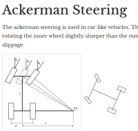 As you can see from the differential equations, we have not only state variables (vector x) but also control variables. Control variables (vector u) describe the inputs to your system.

Example for a car:
control vector: [a, delta]

Using the control vector u,  the state vector x and the ODE, you can compute (or predict) the outputs  of the system (or process) for the next time step. The output is again a vector containing the changed state variables. The process (the car in this case) transforms the input state with the control inputs into the output state.

control input u —> process (input state x, ODE) —> output state x

The ‘job’ of the controller is now to find the optimal control input u that results in an output state that is as close as possible to some reference state at each time step. Or in other words, the controller tries to minimize the error between process output and reference variables via the control input variables for T time steps (this can be seen as an ‘optimization problem’).

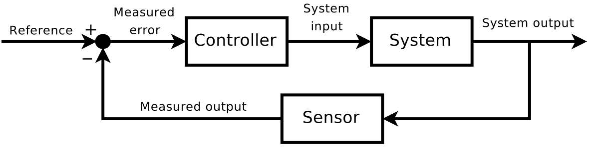
Because the input is more than one variable (a state vector containing multiple variables) and the output is again a state vector, the controller is called Multi-Input-Multi-Output (MIMO). If the output state (or sensor output for a real process) of the system is feed back to the controller and compared to some reference state vector, the controller is called closed-loop.

In all example code, we will need to store more than one state vector (e.g.  over some time steps T) and we will use a matrix to store more than one state:
example states [z0 (x0,y0,v0,phi0), z1 (x1,y1,v1,phi1), z2, etc.] stored in matrix Z:

           |x0,     x1,   x2, ... |
       Z = |y0,     y1,   y2, ... |
           |v0,     v1,   v2, ... |
           |phi0, phi1, phi2, ... |

Model Predictivate Control (MPC)

Model-predictive control (aka as ‘optimal control’) is a control method that tries to compute the optimal control input (u) for some given reference states (Yref), so that your process will output the reference states. However, to correctly predict your process, the MPC controller uses the control input of the past to predict the next states, and a prediction model of the process (the differential equations of the model) as well as a cost matrix (describing which variables of the reference states are more/less important) and optional constraints (e.g. describing the limits of the control input).

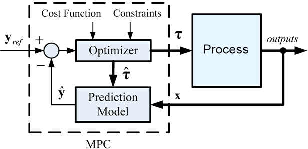
Although the MPC solver will compute the optimal control input for all reference states (prediction horizon), in an MPC closed-loop controller you only apply the first calculated control input (u0) to your process (control horizon). Then you measure your process outputs, find out your reference states, and the whole MPC control starts again.

ACADO Toolkit

We will use the ACADO toolkit (Toolkit for Automatic Control and Dynamic Optimization) to generate fast C code for the MPC controller.

Let’s describe our state variables,  control inputs, differential equations and some constraints for the ACADO toolkit:

// — state variables (acadoVariables.x)—
DifferentialState x;
DifferentialState y;
DifferentialState v;
DifferentialState phi;
// — control inputs —
Control a;
Control delta;
// —- differential equations —-
double L = 1.32;      // vehicle wheel base
DifferentialEquation f;
f << dot(x) == v*cos(phi);
f << dot(y) == v*sin(phi);
f << dot(v) == a;
f << dot(phi) == v*tan(delta)/L;
// — reference functions (acadoVariables.y) —
Function rf;
Function rfN;
rf  << x << y << v << phi;
rfN << x << y << v << phi;
// — constraints, weighting matrices for the reference functions —
// N=number of prediction time steps, Ts=step time interval
// Provide defined weighting matrices:
BMatrix W = eye<bool>(rf.getDim());
BMatrix WN = eye<bool>(rfN.getDim());
// define real-time optimal control problem
OCP ocp(0, N * Ts, N);
ocp.subjectTo( f );
ocp.subjectTo( -1 <= a <= 1 );
ocp.subjectTo( -M_PI <= delta <= M_PI );
ocp.minimizeLSQ(W, rf);
ocp.minimizeLSQEndTerm(WN, rfN);
// — generate MPC code —
OCPexport mpc( ocp );
mpc.exportCode();

Basically, that’s it. In the download below you can find the full code (simple_mpc.cpp). The next step is to compile the code. First, clone the ACADO toolkit, then replace the simple_mpc.cpp in ‘ACADOtoolkit/examples /getting_started/’ by the new one from the download below and compile everything with ‘make’ (works with both Linux and Windows/Visual Studio).

git clone https://github.com/acado/acado.git -b stable ACADOtoolkit
cd ACADOtoolkit
mkdir build
cd build
cmake ..
make

After the code is compiled and the executable is started, the ACADO executable will generate the MPC controller C code for your MPC problem (acado_solver.c, acado_integrator.c, etc).

./simple_mpc

For more details about ACADO, have a look at the tutorials.

Python Extension

We will use a Python C extension (acado.c in download below) to access the ACADO generated C code via Python. This Python Extension code basically converts the Python matrices into C matrices, calls the ACADO generated code, and converts the C matrices back to Python.

(in this example) ACADO uses for each time step the following matrices:

x0:  The initial state of the system (e.g. the current car state)
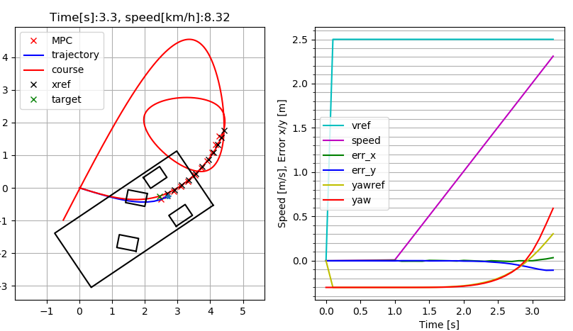
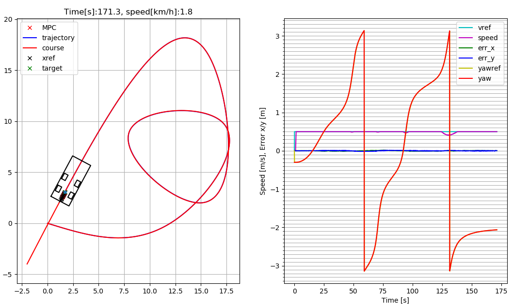
X:   The predicted states of the system for the next (T) prediction time steps using the last control input (u)  (the red crosses in the drawing)
Y:  The reference states of the system for the next (T) prediction time steps (the black crosses in the drawing)
yN:  The final reference state of the system
Q:  A reference states cost matrix for the the next (T) prediction time steps
Qf:  A reference state cost matrix for the final state
constraints: some hard-coded constraints (see ACADO code)
U:  The returned (optimal) control input that controls your process into the reference states (acceleration, steering angle)

The blue dot is the control point (position) of the vehicle. In this example, the steering of the vehicle is at the rear wheel, so the control point is between the front wheels.

To compile the Python extension for your ACADO generated code:

sudo python3 setup.py build install --force

Note: For Windows users, it is recommended to install Anaconda. Then create a new Anaconda Python environment and install the Windows compiler toolchain (‘m2w64-toolchain’ ). See ‘setup.py’ in the download for details.

Python MPC control simulation

Back to the original AtsushiSakai Python Robotics example (‘model_predictive_speed_and_steer_control.py‘).  The Python example steers a car along a reference course. We will replace the non-realtime MPC solver (CVXPY) in the original code with our ACADO Python extension.

The ACADO expects the state variables in the matrix columns, and the states for the T times in the rows. That’s the reason why we transpose all matrices before calling the Python acado.mpc function.

x0, x1, x2 --> x0, y0, ...
y0, y1, y2 --> x1, y1, ...
.., .., ..     x2, y2, ...

For the final result please have a look at the download. Run the demo with:

python3 model_predictive_control2.py

Here’s the result of the simulation (the simulation actually can work much faster than realtime). The black crosses show the reference states, the red crosses the predicted states.

https://youtu.be/_YH3b6Cv7T4

Download

• acado_mpc_python
• mpc_acado_python_deltarate_control (variant where the control is ‘acceleration and delta rate’, so steering angle change and no absolute steering angle)

Where to go from here

• Play with the cost matrices (Q, Qf) and MPC prediction horizon length (T) – you can fine-tune your MPC controller with them!
• Use MPC constraints to add obstacles – your robot will find its way around them!
• In the case you want to play with the ACADO code generator and look for some compilation automation, you can look into the Windows batch / Linux bash files ( model_predictive_control.bat ) to get some ideas.
• You may fine-tune your model (aka ‘system identification’) so it better reflects your physical robot:
  • Python Control Systems Library
  • Systems Identification Package for Python

General issues

• I could not yet manage to add a cost weight for the ‘delta rate of change‘ to ACADO (to reduce the steering angle actions). It complains with everything I try. If you can manage it, please let me know how you did it!
• If I increase simulator frequency (e.g. to 100 Hz), but keep MPC control frequency fixed (e.g. at 10 Hz) something interesting happens: the steering starts to swing. Then I noticed that by using a higher frequency for the model, the speed (v) does not make ‘steps’ but instead smoothly increases (as in reality). Finally, after e.g. 1/100 second this makes already a difference in 5cm between simulation and control model. How should this be fixed? I fixed it by reducing the prediction time horizon (T). If you have any further ideas, please let me know 🙂