Category Archives: Computer Vision

computer vision (stereo vision and other) with MATLAB and C

Kameraposititionssteuerung via Internet

Endlich mal wieder ein kleines Projekt, welches viele Dinge der Informatik miteinander verbindet: Servos, Mikrocontroller, USB-Kamera, Mikrocontroller <-> PC-Kommunikation, HTTP-Server, Javascript, AJAX, Python …

wwwspy

Aber jetzt erstmal im Detail:

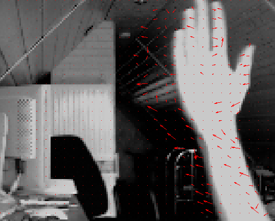
Wie der Titel schon andeutet, geht es darum, eine USB-Webcam, welche auf zwei Servos montiert wurde via einem Web-Interface fernzusteuern – und natürlich das Bild der Kamera zu übertragen.

Das Projekt ist ähnlich dem Projekt von Tobias Weis – allerdings wird hier Windows und als Skriptsprache Python (statt Linux und PHP) verwendet.

Funktionsweise

Die Servos werden über Pulsweitenmodulation (PWM) vom Mikrocontroller angesteuert, der Mikrocontroller erhält die Steuerbefehle via RS232-Schnittstelle (RS232 through USB).  Ein auf dem PC laufender und in Python geschriebener Web-Server liest regelmäßig Bilder von der USB-Kamera, nimmt Befehle vom Web-Client entgegen (Kamera nach rech/links/oben/unten) und schickt diese Befehle dann an den Mikrocontroller.

Benötigte Hardware

  • Mikrocontroller Atmel ATMEGA8L (ich verwende das myAVR Board MK2 USB von myAVR) – dieses Board enthält den Mikrocontroller sowie einen Programmer zum Übertragen der Software in den Mikrocontroller via USB.
  • 2 handelsübliche Servos (werden im Modellbau eingesetzt und gibt es teilweise recht günstig bei eBay – ansonsten beim Modellbauer, Conrad, …)
  • USB-Webcam (gibt’s überall)
  • Ein Netzteil (5V, ca. 1A) zur Energieversorgung der Servos

Benötigte Software

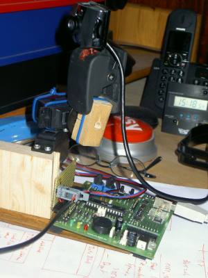
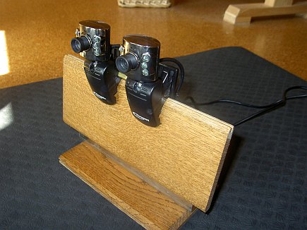
Schritt 1: Servos montieren und mit Mikrocontroller verbinden

Den ersten Servo auf ein Brett fixieren, den zweiten Servo auf den ersten montieren und die Kamera auf den zweiten Servo befestigen. Dann die Steuerleitungen der Servos mit den Atmel Pins PB1 (OC1A) und PB2 (OC1B) verbinden. Zuletzt die +5V und Masse-Leitung der Servos mit dem externen Netzteil verbinden und die Masse-Leitung des externen Netzteils mit der Masse des Atmels verbinden (siehe auch das Schaltbild von Tobias).

Schritt 2: Mikrocontroller programmieren

Als nächstes wird der Atmel-Mikrocontroller programmiert. Zunächst sicherstellen dass die Fuse Bits des Atmels so eingestellt sind, dass dieser mit dem externen 3.6864 Mhz Quartz arbeitet (wichtig für die RS232 Kommunikation), z.B. mit dem Tool AVROSPII. Dann die Mikrocontroller-Software (avr/test2.c bzw. Projektdatei avr/test2.aps) in den Atmel mit AVR Studio übertragen (Build->Build und danach Tool-AVR Prog). Falls das myAVR-Board nicht gefunden wird, überprüfen ob COM1 oder COM2 für den USB-Treiber (->Gerätemanager) verwendet wird.

Nach erfolgereicher Übertragung der Mikrocontroller-Software kann man die Servos mit der Batch-Datei (avr/term.bat) austesten, welche ein RS232-Terminal startet. Durch Drücken der Tasten 1, 2, 3 oder 4 kann man die Servos steuern (rechts/links/oben/unten).

Schritt 3: Web-Server starten

Die WebCam mit dem PC verbinden. Dann den Web-Server starten (im Verzeichnis control ausführen:  python start.py). Nach ein paar Sekunden läuft der Web-Server dann auf Port 8080. Im Web-Browser gibt man also “http://localhost:8080” als URL ein und mit ein bisschen Glück sieht man das Web-Interface der Steuerungssoftware.

Download der Software

Obstacle avoidance in flight via optical flow

This video shows our prototyped flight simulation and controller software that

  1. simulates the flight dynamics of an RC aircraft and
  2. automatically controls that aircraft so that it avoids obstacles (ground/mountains etc.), only by analysing the optical flow in front of the aircraft. For the optical flow sensor, an optical mouse CCD (20×20 pixels) with a lense is simulated.  

Also click here to see how the same technique is used in 2D to navigate a robot, only by optical flow. 

Optical flow based robot obstacle avoidance with Matlab

This is the result of a project where a virtual robot avoids obstacles in a virtual environment without knowing the environment – the robot navigates autonomously, only by analysing it’s virtual camera view.

In detail, this example project shows:

1. How to create a virtual environment for a virtual robot and display the robot’s camera view
2. Capture the robot’s camera view for analysing
3. Compute the optical flow field of the camera view
4. Estimate Focus of expansion (FOE) and Time-to-contact (TTC)
5. Detect obstacles and make a balance decision (turn robot right/turn left)

Matlab’s Virtual Reality toolbox makes it possible to not only visualize a virtual world, but also capture it into an image from a specified position, orientation and rotation. The virtual world was created in VRML with a plain text editor and it can be viewed in your internet browser if you have installed a VRML viewer (you can install one here).

Virtual world for the robot

(Click here to view the VRML file with your VRML viewer) .

For calculating the optical view field of two successive camera images, I used a C optimized version of Horn and Schunk’s optical flow algorithm – see here for details).

Based on this optical flow field, the flow magnitudes of right and left half of each image is calculated. If the sum of the flow magnitudes of the view reaches a certain threshold, it is assumed there is an obstacle in front of the robot. Then the computed flow magnitude of right and left half image is used to formulate a balance strategy: if the right flow is larger than the left flow, the robot turns left – otherwise it turns right.

 Virtual robot GUI

Robot’s camera view at the same time:

Virtual robot camera view

Click here to see a video recording of a robot session. 

Click here to download Matlab code.

Real-time optical flow with Matlab

Did you know that a fly cannot see real stereo? It sees two “images” that have only a small area of the same visual field. So the fly cannot estimate distances by using stereo images, it detects obstacles by “optical flow”. Optical flow is the perceived visual motion of objects as the observer (here the fly) moves relative to them.

I have experimented with optical flow code (based on Horn and Schunck’s optical flow algorithm) these days, and I could manage to visualize the optical flow with it in real-time using 100% Matlab code. The code uses a camera (320×240 pixels) for capturing real-time image frames, computes the optical flow field with the current and the last frame (also called image velocity field) and shows the field in the image.

Optical flow screenshot

The field is calculated for each pixel of the image. The angle of the arrow shows in which direction the specified pixel was moved, the distance shows how much that pixel did move.

How can this optical flow field be used? Well, you could e.g. use the field to estimate the distance to obstacles for a moving vehicle when mounted a camera on it. A nice approach of detecting obstacles for a robot vehicle 🙂

Here’s the Matlab code to download (ovcam.zip).

USB stereo camera evaluation project

The aim of this project is to experiment with a self-made USB stereo vision camera system to generate a depth-map image of an outdoor urban area (actually a garden with obstacles) to find out if such a system is suitable for obstacle detection for a robotic mower. The USB camera I did take (Typhoon Easycam 1.3 MPix) is very low priced (~12 EUR) and this might be the cheapest stereo system you can get.stereocam.jpg

For the software, the following steps are involved for the stereo vision system:

1. Calibrate the stereo USB cameras with the MATLAB Camera Calibration Toolbox to determine the internal and external camera paramters. The following picture shows the snapshot images (left camera) used for stereo camera calibration.
calibimages.jpg

2. Use these camera paramters to generate rectified images for left and right camera images, so that the horizontal pixel lines of both cameras contain the same obstacle pixels. Again, the mentioned calibration toolbox was helpful to complete this task since rectification is included.3. Find some algorithm to find correlations of pixels on left and right images for each horizontal pixel line.This is the key element of a stereo vision system. There are algorithms that produce accurate results and they tend to be slow and often are not suitable for realtime applications. For my first tests, I did experiment with the MATLAB code for dense and stereo matching and dense optical flow of Abhijit S. Ogale and Justin Domke whose great work is available as open-source C++ library (OpenVis3D). Running time for my test image was about 4 seconds (1.3 GHz Pentium PC).4. Compute the disparity map based on correclated pixels.My test image:
sample1.jpg

The disparity map generated (from high disparity on red pixels to low disparity on blue pixels):

depthmap.jpg

The results are already impressive – future plans involve finding faster algorithms, maybe some idea that solves the problem in another way. Finding a quick way to find matches (from left to right) in intervals between the left and right intensity scan lines for each horinzontal pixel line could be a solution, although it might always be too slow for realtime applications.

intensitymatch.jpg


Update (06-17-2009):
  I have been asked several times now how exactly all steps are performed. So, here are the detailed steps:

  1. Learn how to use the calibration toolbox using one camera first. I don’t know how to calibrate the stereo-camera system without the chessbord image (anyone knows?), however it is very easy to create this chessboard image – download the .PDF file, print it out (measure the box distances, vertical and horizontal line distances in each box should be the same), and stick it onto a solid board. Calibrate your stereo-camera system to compute your camera parameters. A correct calibration is absolutely necessary for the later correlation computation. Also, check that the computed pixel reprojection error after calibration is not too high (I think mine was < 1.0). After calibration, you’ll have a file “Calib_Results_stereo.mat” under the snapshots folder. This file contains the computed camera paramters.
  2. Now comes the tricky part 😉 – In your working stereo camera system, for each two camera frames you capture (left and right), you need to rectify them using the Camera Calibration Toolbox. You could do this using the function ‘rectify_stereo_pair.m’ – unfortuneately, the toolbox has no function to compute the rectified images in memory, so I did modify it – my function as well as my project (stereocam.m) is attached.Call this at your program start somewhere:
    rectify_init

    This will read in the camera parameters for your calibrated system (snapshots/Calib_Results_stereo.mat) and finally calculate matrices used for the rectification.
  3. Capture your two camera images (left and right).
  4. Convert them to grayscale if they are color:
    imL=rgb2gray(imL)
    imR=rbg2gray(imR)
  5. Convert the image pixel values into double format if your pixel values are integers:
    imL=double(imL)
    imR=double(imR)
  6. Rectify the images:
    [imL, imR] = rectify(imL, imR)
  7. For better disparity maps, crop the rectified images, so that any white area (due to rotation) is cropped from the images (find out the cropping sizes by trial-and-error):
    imL=imcrop(imL, [15,15, 610,450]
    imR=imcrop(imR, [15,15, 610,450]
  8. The rectified and cropped images can now be used to calculate the disparity map. In my latest code, I did use the ‘Single Matching Phase (SMP)’ algorithm from Stefano, Marchionni, Mattoccia (Image and Computer Vision, Vol. 22, No .12):
    [dmap]=VsaStereoMatlab(imL’, imR’, 0, Dr, radius, sigma, subpixel, match)
  9. Do any computations with returned depth map, visualize it etc.

And finally, here’s the Matlab code of my project (without the SMP code).