Did you know that a fly cannot see real stereo? It sees two “images” that have only a small area of the same visual field. So the fly cannot estimate distances by using stereo images, it detects obstacles by “optical flow”. Optical flow is the perceived visual motion of objects as the observer (here the fly) moves relative to them.
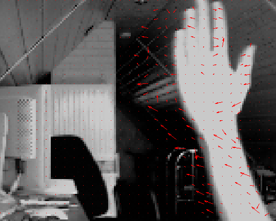
I have experimented with optical flow code (based on Horn and Schunck’s optical flow algorithm) these days, and I could manage to visualize the optical flow with it in real-time using 100% Matlab code. The code uses a camera (320×240 pixels) for capturing real-time image frames, computes the optical flow field with the current and the last frame (also called image velocity field) and shows the field in the image.
The field is calculated for each pixel of the image. The angle of the arrow shows in which direction the specified pixel was moved, the distance shows how much that pixel did move.
How can this optical flow field be used? Well, you could e.g. use the field to estimate the distance to obstacles for a moving vehicle when mounted a camera on it. A nice approach of detecting obstacles for a robot vehicle 🙂
Habe Sie sich schon einmal irgendwo angemeldet, damit Sie ein (scheinbar kostenloses) Internet-Angebot nutzen können? Haben Sie danach eine Rechnung und anschließende Mahnungen erhalten? Nein? Mir ist dies wie vielen anderen tausenden Internet-Benutzern nun passiert. Die Masche ist scheinbar seit langem bekannt und die Machart des Drahtziehers ist immer dieselbe:
Man muss sich anmelden und die AGB bestätigen, um eines der vielen (scheinbar kostenlosen) Internet-Angebot des dubiosen Anbieters nutzen zu können.
Die eigentlich wichtige Information, dass das Angebot gebührenpflichtig ist, findet sich unterhalb der Internet-Seite an einer Stelle (im Kleingedruckten), die man u.U. gar nicht zu Gesicht bekommt.
Nach der Anmeldung erhält man keine weitere unmittelbare Mitteilung darüber, dass man soeben einen Vertrag abgeschlossen hat. Diese Information ist einzig und allein in den AGB versteckt.
Nach Ablauf einer Kündigungsfrist (die einem ebenfalls nicht direkt mitgeteilt wird, sondern sich in den AGB versteckt), erhält man zunächst eine Rechnung, dann eine Mahnung, dann eine zweite Mahnung, dann ggf. ein Inkassoschreiben, dann ggf. Schreiben von Anwälten.
Man bedenke, dass dies ein vollständiges “Geschäftsmodell” für den Abzocker darstellt – falls auch nur einige “Betroffene” zahlen, ist die Kasse gefüllt, um weitere Leute zu verunsichern und abzumahnen. Da es immer einige Leute gibt, die der Zahlung nachkommen werden, geht die Rechnung leider auf und der Abzocker kann seinem Geschäft weiter nachgehen und dieses ausbauen.
Bei einem genaueren Blick sollte einem dieses Geschäftsmodell jedoch als grenzwertig kriminell auffallen. Enstprechende Urteile des Amtsgerichts München (AZ 161 C 23695/06) und des Amtsgerichts Hamm (AZ 17 C 62/08) belegen, dass man vort Gericht mit sehr hoher Wahrscheinlichkeit gewinnt, allerdings wird es in 99,9999% der Fälle gar nicht soweit kommen, da dann das Geschäftsmodell des Abzockers offiziell als rechtswidrig bestätigt werden würde.
Daher bleibt einem nur, folgende Punkte zu beachten:
Auf keinen Fall zahlen.
Unmittelbar der Rechnung per Brief (Einschreiben) widersprechen. Die Verbraucherzentralen bieten hierfür Musterschreiben an.
Alle Beweismittel sammeln (Screenshots des Internet-Angebots, E-Mails, Briefe).
Briefe von Anwälten und Inkassofirmen ignorieren.
Falls es wirklich zu einem *gerichtlichen* Mahnbescheid kommt, diesem widersprechen.
Damit ist die Sache in 99,9999% der Fälle erledigt. Der dubiose Internet-Anbieter wird in keinem Fall die seine Aktivitäten fortsetzen und einen Prozess anstreben, da er diesen ggf. verlieren würde, das werden auch die Verbraucherzentralen und Anwälte bestätigen.
Ich hoffe, ich konnte ein hiermit beitragen, ein wenig Licht ins Dunkel der dubiosen Internet-Geschäftemacher zu bringen. Es bleibt zu hoffen, dass dieses Geschäftsmodell zukünftig nicht noch mehr Nachahmer finden wird bzw. dass das Internet-Dienstleistungsgeschäft durch neuere Rechtssprechnung für den Kunden transparenter und sicherer wird!
Vorsicht! Die Kreativität dieser dubiosen Internetdienstleister kennt keine Grenzen – schon morgen könnte man selbst in eine andere Falle tappen 😉
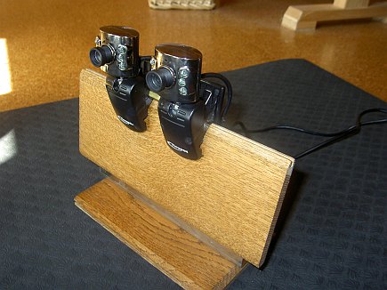
The aim of this project is to experiment with a self-made USB stereo vision camera system to generate a depth-map image of an outdoor urban area (actually a garden with obstacles) to find out if such a system is suitable for obstacle detection for a robotic mower. The USB camera I did take (Typhoon Easycam 1.3 MPix) is very low priced (~12 EUR) and this might be the cheapest stereo system you can get.
For the software, the following steps are involved for the stereo vision system:
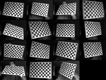
1. Calibrate the stereo USB cameras with the MATLAB Camera Calibration Toolbox to determine the internal and external camera paramters. The following picture shows the snapshot images (left camera) used for stereo camera calibration.
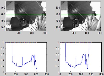
2. Use these camera paramters to generate rectified images for left and right camera images, so that the horizontal pixel lines of both cameras contain the same obstacle pixels. Again, the mentioned calibration toolbox was helpful to complete this task since rectification is included.3. Find some algorithm to find correlations of pixels on left and right images for each horizontal pixel line.This is the key element of a stereo vision system. There are algorithms that produce accurate results and they tend to be slow and often are not suitable for realtime applications. For my first tests, I did experiment with the MATLAB code for dense and stereo matching and dense optical flow of Abhijit S. Ogale and Justin Domke whose great work is available as open-source C++ library (OpenVis3D). Running time for my test image was about 4 seconds (1.3 GHz Pentium PC).4. Compute the disparity map based on correclated pixels.My test image:
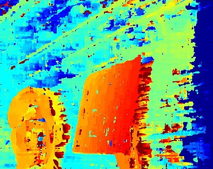
The disparity map generated (from high disparity on red pixels to low disparity on blue pixels):
The results are already impressive – future plans involve finding faster algorithms, maybe some idea that solves the problem in another way. Finding a quick way to find matches (from left to right) in intervals between the left and right intensity scan lines for each horinzontal pixel line could be a solution, although it might always be too slow for realtime applications.
Update (06-17-2009): I have been asked several times now how exactly all steps are performed. So, here are the detailed steps:
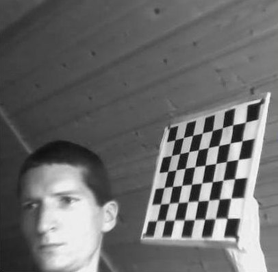
Learn how to use the calibration toolbox using one camera first. I don’t know how to calibrate the stereo-camera system without the chessbord image (anyone knows?), however it is very easy to create this chessboard image – download the .PDF file, print it out (measure the box distances, vertical and horizontal line distances in each box should be the same), and stick it onto a solid board. Calibrate your stereo-camera system to compute your camera parameters. A correct calibration is absolutely necessary for the later correlation computation. Also, check that the computed pixel reprojection error after calibration is not too high (I think mine was < 1.0). After calibration, you’ll have a file “Calib_Results_stereo.mat” under the snapshots folder. This file contains the computed camera paramters.
Now comes the tricky part 😉 – In your working stereo camera system, for each two camera frames you capture (left and right), you need to rectify them using the Camera Calibration Toolbox. You could do this using the function ‘rectify_stereo_pair.m’ – unfortuneately, the toolbox has no function to compute the rectified images in memory, so I did modify it – my function as well as my project (stereocam.m) is attached.Call this at your program start somewhere:
rectify_init
This will read in the camera parameters for your calibrated system (snapshots/Calib_Results_stereo.mat) and finally calculate matrices used for the rectification.
Capture your two camera images (left and right).
Convert them to grayscale if they are color: imL=rgb2gray(imL)
imR=rbg2gray(imR)
Convert the image pixel values into double format if your pixel values are integers:
imL=double(imL)
imR=double(imR)
Rectify the images:
[imL, imR] = rectify(imL, imR)
For better disparity maps, crop the rectified images, so that any white area (due to rotation) is cropped from the images (find out the cropping sizes by trial-and-error): imL=imcrop(imL, [15,15, 610,450]
imR=imcrop(imR, [15,15, 610,450]
The rectified and cropped images can now be used to calculate the disparity map. In my latest code, I did use the ‘Single Matching Phase (SMP)’ algorithm from Stefano, Marchionni, Mattoccia (Image and Computer Vision, Vol. 22, No .12): [dmap]=VsaStereoMatlab(imL’, imR’, 0, Dr, radius, sigma, subpixel, match)
Do any computations with returned depth map, visualize it etc.
And finally, here’s the Matlab code of my project (without the SMP code).
Wouldn’t it be nice to lie in the sun and have a robotic mower mow the lawn (and do the boring work)? Well, at least this is the aim (among other aspects as learning more about designing such systems) of this project…
A) Mechanics
Two wheels of a seed vehicle
Two office chair front wheels
Two DC motors motors (12V, 40W) with gear (23:1)
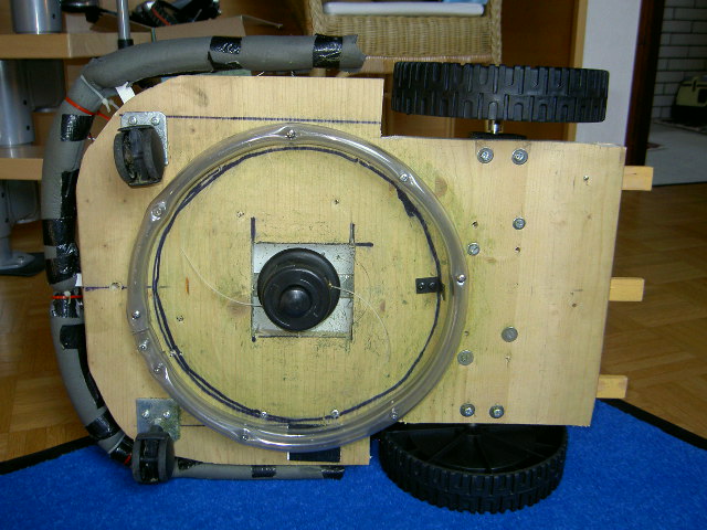
B) Mowing unit
DC motor from a 18V battery lawn trimmer
C) Controller
Microcontroller board ATMEGA168 (myAVR, 50 EUR) for reading the sensors and controlling the motors (two rear motors).
D) Sensors
Three Sharp IR sensors to detect near obstacles
RGB color sensor to detect non-lawn/lawn areas (no need to build a virtual fence in your garden!)
Bumper with three micro switches
E) All other parts
A wooden board (38 x 53 cm) for assembly of everything
Two gel-lead batteries (2 x 12V, 10Ah)
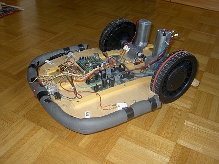
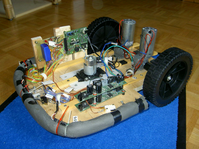
F) First version (without mowing unit), without sensors
Click here to see video (9 MB) which shows this mower prototype in action (indoor) 🙂 G) Second version – now with sensors and mowing unit!
The color sensor is working – the RGB color value is measured periodically and then converted into HSV (hue/saturation/value) color model. A first test with real lawn shows it can detect areas with a green color very precisely. For testing the algorithm, the first goal was to keep the robot on the blue piece of carpet – it successfully stayed on there, even after ‘mowing’ for 30 minutes!
A blog on projects with robotics, computer vision, 3D printing, microcontrollers, car diagnostics, localization & mapping, digital filters, LiDAR and more